To help illustrate the challenge given in this lecture I’ve gone ahead and organised the traversal into a tree diagram. This is a great way to visualised what’s actually going on and should should be particularly helpful for anyone who is struggling to see how the trace back works when you finally reach the goal.
So, the challenge was to manually work out the shortest path for the following grid, using the directional priority; up, right, down, left:
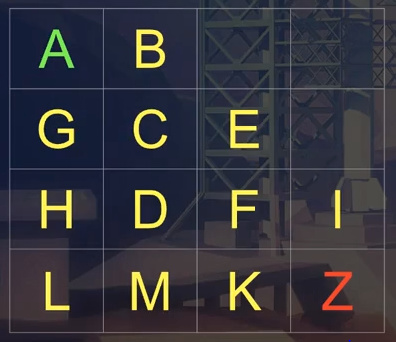
I won’t go into the specifics of how to actually traverse the grid, since Ben already does a fine job at explaining it in the video.
Now, by following the instructions of our algorithm, you’re building a tree that looks something like this:
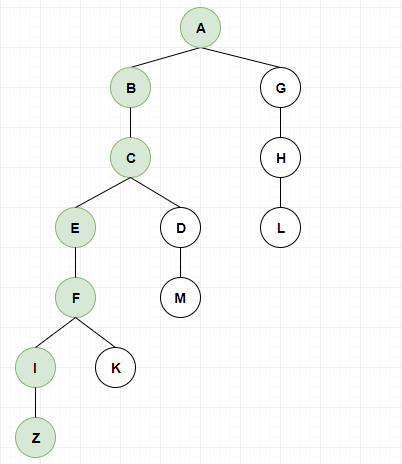
Notice that every time a visited node has somewhere to go, those nodes are added as branches on the tree. However, each node can only be added to the tree once.
This gives us a queue in the order A-B-G-C-H-E-D-L-F-M-I-K-Z.
So to find the path back to the start, all you do is work your way back up the tree.
Therefore, the shortest path (according to our algorithm) is A-B-C-E-F-I-Z.
But what about the other paths we could have taken? What happens if we change the directional priority to favour moving down before moving right?
Well, that’s easy! Here’s the tree for the same grid but searched with the down-right directional priority.
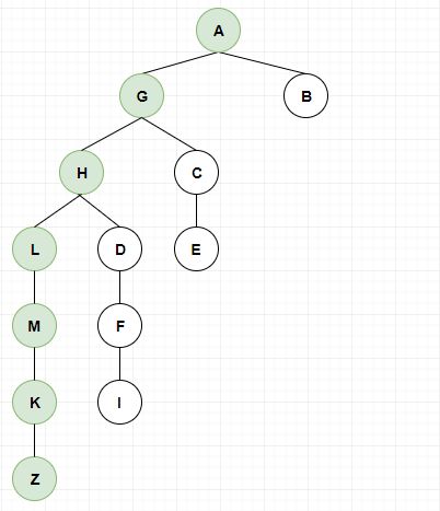
This new tree gives us a queue in the order A-G-B-H-C-L-D-E-M-F-K-I-Z.
So now the path shortest path is (A-G-H-L-M-K-Z)
As you can see this, corresponds to moving straight down on the grid and then moving right.
I hope this helps with your understanding of this breadth first search algorithm.